A Case Study of Bird Richness and Tomb Occupancy in the Thousand Island Lake
Institute of Imagination Sciences, Zhejiang University, Hangzhou Zhejiang 310035, China
Abstract
Because of the biases and shortcomings of the stepwise multiple regression, the Information Theoretic is becoming a reliable method to infer the data, although there are a plethora of candidate models when using Information Theoretic. Here, based on the Akaike Information Criterion, we analysed the determinants of bird richness on islands in the Thousand Island Lake. We also discussed distribution patterns of tombs on study islands using the method of multimodel inference. The results showed bird communities on the islands were determined by island area and habitat richness, whereas the occupancy of tombs was determined by the shape of islands. This is the first evidence showing bird richness significantly related to tomb occupancy. This finding may have potential implications in tomb searchings in the region of the Thousand Island Lake.
Keywords
AIC, model selection, birds, multimodel inference, stepwise regression, Thousand Island Lake, tomb distribution
Introduction
How to choose the most parsimonious (best) model in a large set of competing models in your analyses? Using stepwise multiple regression, or the Information Theoretic Analysis? Whittingham et al. (2006) found 57% of 65 papers published in three leading ecological journals (Ecology Letters, Journal of Applied Ecology, and Animal Behaviour) used a stepwise approach. Although the stepwise regression has several principal drawbacks, such as bias in parameter estimation, inconsistencies among model selection algorithms, an inherent problems of multiple hypothesis testing and an inappropriate focus or reliance on a single best model, it is still widely used. It is out the scope of this paper to detail these shortages of stepwise regression. In this paper, I will introduce how to use the AIC for model selection.
The Thousand Island Lake (hereafter, the Lake) locates at the western Zhejiang Province, eastern China. It was created in 1959 by the construction of Xin’anjiang Dam. Flooding around 500 km^2, it formed 1078 islands with area > 0.25 ha at 108 m water-level, which is a natural experiment for the studying of island biogeography and conservation biology. Our group began to survey the bird communities since 2002, and now expands to many biological taxa, e.g., spiders, reptiles, amphibians, snakes, monkeys, insects, small mammals, butterflies and plants. It is an ongoing and growing project, and we warmly welcome all scientists to join and collaborate in this project. Just several months ago, I talked with the Spiderman Dr. Wu in our group who are the local expert on spiders, and discussed the possibility to analyze the relationship between bird richness and fengshui on our study islands. Yes, I know it is not easy to explain the notion fengshui in English which is one of the traditional Chinese culture. For simplicity, fengshui is analogous to good luck. For example, when someone has passed away, his/her family will try to find some place that have good fengshui to build the tomb and hope he/she will have another good living place after death.
Here, I used the method of model selection and multimodel inference to analyze the determinants of the bird richness and tomb occupancy on the islands in the Lake. This paper addressed following questions: 1) What is the AIC? Does it mean the American International College? 2) What are the key processes to run the multimodel inference? 3) What are the determinants of the bird and tomb distribution on the islands in the Lake.
Materials and Methods
Study area and island attributes
We sampled 40 islands randomly stratified across the area and isolation gradients in the Lake. We measured many island attributes that are related to bird richness in 2002, including area, isolation, plant richness, habitat types, perimeter, perimeter to area ratio (PAR), shape index (SI) and maximum elevation of each island. I also imagined several island attributes that may be related to robbing a grave on the islands, such as convex, slope, aspect, Al, Si, and sand index.
The elements of Al and Si are the main substances of Kaolin clay that is a good type of waterproof soil for tomb buildings. The sand index is an indicator of tomb occurrence on the island, because it is impossible to find a tomb in an area that is full of sand. The pH value is an indicator of organic materials in the tomb. Other factors, e.g. SI, convex, slope and aspect, are the useful indicators of fengshui. For example, a mountain with its shape in a perfect circle, with thick soil and high plant richness will be the priority place to set a tomb.
AIC
AIC (Akaike Information Criterion) measures the relative quality of a statistical model, for a given set of data. AIC is based on information entropy, so that it does not provide a test of a model, i.e. testing a null hypothesis. In this way, AIC can tell nothing about the quality of the model in an absolute sense. If all candidate models are fitted poorly, AIC will not give any warning of that.
Basically, AIC is
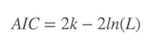
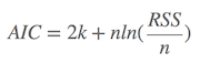
where k is the number of parameters in the model, L is the maximized value of the likelihood function of the model. Several existing functions in R packages were already developed, such as AIC function in stat package, and extractAIC in stats package to calculate the AIC values. If you would like to calculate the AIC values by yourself, it is also easy to make it. Suppose the variance of the model distributes is normal, and n is the number of sampling, RSS is the residual-sum-squares, so
Given a set of candidate models for the data, the preferred model is the one with the minimum AIC value. Hence, AIC not only rewards goodness of fit, but also includes a penalty that is an increasing function of the number of estimated parameters. This penalty discourages overfitting.
When the sample size (n/k) < 40, the AIC is corrected by AICc (corrected AIC)
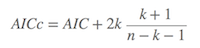
where n denotes the sample size. Burnham & Anderson (2002) strongly recommend using AICc, rather than AIC when n is small or k is larger. Because AICc converges to AIC as n is being larger, AICc generally should be the first choice for model selection (Note: most of the contents in this section was borrowed from Wikipeadia, whereas the year of the Burnham & Anderson’s book should be 2002, not 2004 as showed in the Chinese version of this page).
If the overdispersion exists in the data, the QAIC would be the better choice, which is
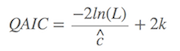
$\hat{c}$ is the variance inflation factor, or the overdispersion coefficient. If $\hat{c}$ > 1, the QAIC should be used.
Calculating the model weights
Once we calculated the AIC values for each model, these models were sorted in the decreasing order of AIC values. ∆AIC represents the AIC value of each model minus the smallest one in the set of models. The model weight, also called Akaike weight(wi), is calculated as
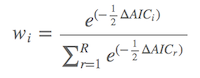
where wi the weight of the ith model. wi ranges between 0 and 1, and the sum of them equals 1. The larger the model weights, the more possibilities to be the best “true” model. For example, if we have a model with the model weight w2 of 0.31, indicating the probability of this model to be the best “true” model is 31%.
The relative importance of each parameter can be calculated by the model weights, which added the weights of the model containing the parameter. After ranking the importance in the decreasing order, it is clear which parameter has the largest importance.
Model selection uncertainty and multimodel inference
In practice, the result will be not so perfect as expected. All previous results were based on the assumption of ∆AIC > 2, meaning the difference of the AIC between the first and second best model is more than 2. If ∆AIC > 2, it is safe to use the first model as the best model. If not, it means the first several competing models have substantially supported. So, how to deal with this trick when ∆AIC of the first two best model < 2? The terminal weapon is model averaging.
∆AIC > 2 is considered as a golden rule in model selection (Burnham & Anderson, 2002). However Anderson (2008) suggested it is better to include all candidate models into model selection UNLESS some models should be removed for confidence reasons. We know that models with low AIC values will also have low model weights, so the model-averaged result will not be influenced very much if these models were included. Suppose Y^ is the observed dependent value, e.g. the bird richness or the occupancy of the tomb in this case, which is estimated as
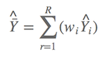
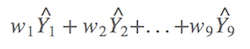
It means if you have nine candidate models, there are nine model weights, and could produce nine observes. The model-averaged prediction is the summed product of each prediction by its model weight,
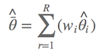
Similar as the model-averaged prediction, we can also calculate the model-averaged estimates of parameters. Suppose the estimate of the ith parameter is θi, it can be calculated directly from the model with the smallest AIC value if the ∆AIC > 2. If ∆AIC < 2, the averaged estimate of parameter is given by
With the model weight, we obtained the unconditional variance estimate (Burnham & Anderson, 2002, p.162)
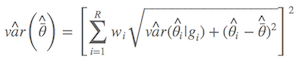
Dr. Anderson suggested we should use the alternative one (Anderson, 2008, p.111), which is
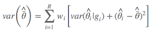
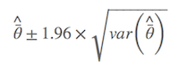
where $\hat{\bar{θ}}$ is the model-averaged estimate, wi is model weight, and gi is the ith model. As described by Anderson (2008), an estimator of the variance of parameter estimator estimates that incorporates both sampling variance, given a model, and a variance component for model selection uncertainty. As a result, the confidence interval is
Case study
Before running the following code, it is essential to be sure that these packages (glmulti, MuMIn, bbmle) were installed. If not, simply entering the line of the code below into the R console to start the installation automatically.
install.packages("glmulti")The alternative method to install these packages is to download them from any CRAN of R project to your computer, and then install them locally.
Case One: the determinant of bird richness in the Lake
Load glmulti package
library(glmulti)## Loading required package: rJava
Load the bird and island data (this is the real data, but I shuffled them randomly)
tilbird <- read.table("http://sixf.org/files/code/2014/tilbird.txt", h = T)  #find 'tilbird.txt' and open it
str(tilbird)  # check the data structure of `til.bird`
## 'data.frame': 40 obs. of 9 variables:
## $ birdspp : int 43 34 35 32 31 27 30 33 24 24 ...
## $ area : num 1289.2 143.2 109 55.1 46.4 ...
## $ isolation: num 897 1415 965 954 730 ...
## $ plants : int 36 50 88 86 65 68 45 49 45 31 ...
## $ habitats : int 3 6 3 3 3 3 3 7 4 4 ...
## $ Pe : num 105965 17465 12022 7570 10444 ...
## $ PAR : num 82.2 122 110.3 137.4 225.2 ...
## $ SI : num 832 412 325 288 433 ...
## $ elev : num 298 251 227 198 174 ...
The first column of the data is the bird species on each island, and thereby eight island attributes, which are the area, isolation, plant richness, habitat types, perimeter, PAR, SI and elevation. Larger PAR indicates more edges comparing the interior area of an island. SI will be 1 if the island is a perfect circle.
Before running the model, we should check the independence of each variable. There are several available methods, such as correlation test, VIF and PCA analyses. Here, we use the common method: the correlation test.
The R function for correlation test is cor.test, which is a test for two vectors. Function cor can run the correlation with more than two vectors, but no p-values showed in the result. To overcome the shortage of these two functions, I wrote a simple function to run the test with a p-value in the result, named cor.sig.
cor.sig = function(test) {
    res.cor = cor(test)
    res.sig = res.cor
    res.sig[abs(res.sig) > 0] = NA
    nx = dim(test)[2]
    for (i in 1:nx) {
        for (j in 1:nx) {
            res.cor1 = as.numeric(cor.test(test[, i], test[, j])$est)
            res.sig1 = as.numeric(cor.test(test[, i], test[, j])$p.value)
            if (res.sig1 <= 0.001) {
                sig.mark = "***"
            }
            if (res.sig1 <= 0.01 & res.sig1 > 0.001) {
                sig.mark = "** "
            }
            if (res.sig1 <= 0.05 & res.sig1 > 0.01) {
                sig.mark = "*  "
            }
            if (res.sig1 > 0.05) {
                sig.mark = "   "
            }
            if (res.cor1 > 0) {
                res.sig[i, j] = paste(" ", as.character(round(res.cor1, 3)),
                  sig.mark, sep = "")
            } else {
                res.sig[i, j] = paste(as.character(round(res.cor1, 3)), sig.mark,
                  sep = "")
            }
        }
    }
    as.data.frame(res.sig)
}
Put all island attributes into the correlation test,
cor.sig(tilbird[, 2:9]) # exclude the first column which is the bird richness, the Y values.## area isolation plants habitats Pe PAR
## area 1*** -0.115 -0.139 -0.064 0.996*** -0.429**
## isolation -0.115 1*** -0.101 -0.1 -0.117 0.299
## plants -0.139 -0.101 1*** -0.16 -0.138 -0.048
## habitats -0.064 -0.1 -0.16 1*** -0.057 -0.035
## Pe 0.996*** -0.117 -0.138 -0.057 1*** -0.481**
## PAR -0.429** 0.299 -0.048 -0.035 -0.481** 1***
## SI 0.857*** -0.045 -0.167 -0.034 0.898*** -0.619***
## elev 0.726*** -0.127 -0.039 -0.032 0.775*** -0.803***
## SI elev
## area 0.857*** 0.726***
## isolation -0.045 -0.127
## plants -0.167 -0.039
## habitats -0.034 -0.032
## Pe 0.898*** 0.775***
## PAR -0.619*** -0.803***
## SI 1*** 0.888***
## elev 0.888*** 1***
The results indicated significant correlations among area, perimeter, PAR, SI and elevation. We know area is a very important parameter in the theory of island biogeography. Other parameters may result by area, so I dropped the perimeter: PAR, SI and elevation, and kept four parameters: area, isolation, plant richness and habitat types for the analyses.
I simply chose the linear model for the dataset, so the global model is
global.model <- lm(birdspp ~ area + isolation + plants + habitats, data = tilbird)Then I used the function glmulti in the glmulti package to check the ‘best ‘ model whose AIC is smallest. Because I have four parameters, it will totally have 2^4=16 candidate models. Here, the interaction effects between island attributes were not addressed.
bird.model <- glmulti(global.model, level = 1, crit = "aicc") # use the AICc to choose the model because it works better in small samples## Initialization...
## TASK: Exhaustive screening of candidate set.
## Fitting...
## Completed.
summary(bird.model)## $name
## [1] "glmulti.analysis"
##
## $method
## [1] "h"
##
## $fitting
## [1] "lm"
##
## $crit
## [1] "aicc"
##
## $level
## [1] 1
##
## $marginality
## [1] FALSE
##
## $confsetsize
## [1] 100
##
## $bestic
## [1] 223.7
##
## $icvalues
## [1] 223.7 223.8 225.0 225.7 226.2 226.7 228.6 228.7 243.6 244.1 244.5
## [12] 244.5 246.0 246.7 246.8 247.0
##
## $bestmodel
## [1] "birdspp ~ 1 + area + habitats"
##
## $modelweights
## [1] 2.871e-01 2.708e-01 1.455e-01 1.049e-01 8.123e-02 6.348e-02 2.432e-02
## [8] 2.259e-02 1.332e-05 1.036e-05 8.538e-06 8.461e-06 3.984e-06 2.794e-06
## [15] 2.652e-06 2.496e-06
##
## $includeobjects
## [1] TRUE
The result came out. The best model retained the variables of area and habitat types. Now I will check all possible models one by one and find the best one.
lm9 <- lm(birdspp ~ area + habitats, data = tilbird)
summary(lm9)
##
## Call:
## lm(formula = birdspp ~ area + habitats, data = tilbird)
##
## Residuals:
## Min 1Q Median 3Q Max
## -6.606 -2.107 -0.263 1.911 8.705
##
## Coefficients:
## Estimate Std. Error t value Pr(>|t|)
## (Intercept) 20.69295 2.08432 9.93 5.6e-12 ***
## area 0.01564 0.00289 5.41 3.9e-06 ***
## habitats 1.29893 0.55652 2.33 0.025 *
## ---
## Signif. codes: 0 '***' 0.001 '**' 0.01 '*' 0.05 '.' 0.1 ' ' 1
##
## Residual standard error: 3.67 on 37 degrees of freedom
## Multiple R-squared: 0.474, Adjusted R-squared: 0.445
## F-statistic: 16.6 on 2 and 37 DF, p-value: 7e-06
Check the AICc values:
summary(bird.model)$icvalue## [1] 223.7 223.8 225.0 225.7 226.2 226.7 228.6 228.7 243.6 244.1 244.5
## [12] 244.5 246.0 246.7 246.8 247.0
The ∆AICc of the second model is 225.6429-225.4588=0.1841, which is < 2. If the ∆AICc > 2, all analyses of this dataset is completed and selecting the first model with lowest AICc value as the best model. Sadly, it is not! Now, we should run the model averaging, and list all possible models (16 models):
lm1 <- lm(birdspp ~ area + isolation + plants + habitats, data = tilbird)
lm2 <- lm(birdspp ~ isolation + plants + habitats, data = tilbird)
lm3 <- lm(birdspp ~ area + plants + habitats, data = tilbird)
lm4 <- lm(birdspp ~ area + isolation + habitats, data = tilbird)
lm5 <- lm(birdspp ~ area + isolation + plants, data = tilbird)
lm6 <- lm(birdspp ~ plants + habitats, data = tilbird)
lm7 <- lm(birdspp ~ isolation + habitats, data = tilbird)
lm8 <- lm(birdspp ~ isolation + plants, data = tilbird)
lm9 <- lm(birdspp ~ area + habitats, data = tilbird)
lm10 <- lm(birdspp ~ area + plants, data = tilbird)
lm11 <- lm(birdspp ~ area + isolation, data = tilbird)
lm12 <- lm(birdspp ~ area, data = tilbird)
lm13 <- lm(birdspp ~ isolation, data = tilbird)
lm14 <- lm(birdspp ~ plants, data = tilbird)
lm15 <- lm(birdspp ~ habitats, data = tilbird)
lm16 <- lm(birdspp ~ 1, data = tilbird)
Looks crazy? It will be tricky if you have 10 parameters as there are 2^10=1024 candidate models! Take it easy… We can create a loop function and feed it to the computer to run the calculation (not shown here).
Average models together,
library(MuMIn)
lm.ave <- model.avg(lm1, lm2, lm3, lm4, lm5, lm6, lm7, lm8, lm9, lm10, lm11,
    lm12, lm13, lm14, lm15, lm16)
summary(lm.ave)
##
## Call:
## model.avg.default(object = lm1, lm2, lm3, lm4, lm5, lm6, lm7,
## lm8, lm9, lm10, lm11, lm12, lm13, lm14, lm15, lm16)
##
## Component models:
## df logLik AICc Delta Weight
## 12 4 -107.3 223.7 0.00 0.29
## 123 5 -106.0 223.8 0.12 0.27
## 124 5 -106.6 225.0 1.36 0.15
## 1234 6 -105.6 225.7 2.01 0.10
## 13 4 -108.5 226.2 2.53 0.08
## 1 3 -110.0 226.7 3.02 0.06
## 134 5 -108.4 228.6 4.94 0.02
## 14 4 -109.8 228.7 5.08 0.02
## 3 3 -118.5 243.6 19.96 0.00
## 23 4 -117.5 244.1 20.46 0.00
## (Null) 2 -120.1 244.5 20.85 0.00
## 2 3 -118.9 244.5 20.86 0.00
## 34 4 -118.4 246.0 22.37 0.00
## 234 5 -117.5 246.7 23.08 0.00
## 4 3 -120.1 246.8 23.18 0.00
## 24 4 -118.9 247.0 23.31 0.00
##
## Term codes:
## area habitats isolation plants
## 1 2 3 4
##
## Model-averaged coefficients:
## Estimate Std. Error Adjusted SE z value Pr(>|z|)
## (Intercept) 22.023011 3.272613 3.327045 6.62 <2e-16 ***
## area 0.015423 0.002945 0.003044 5.07 <2e-16 ***
## habitats 1.287322 0.560392 0.579478 2.22 0.026 *
## isolation -0.001104 0.000728 0.000753 1.47 0.143
## plants 0.019405 0.021519 0.022247 0.87 0.383
## ---
## Signif. codes: 0 '***' 0.001 '**' 0.01 '*' 0.05 '.' 0.1 ' ' 1
##
## Full model-averaged coefficients (with shrinkage):
## (Intercept) area habitats isolation plants
## 22.023011 0.015422 1.040595 -0.000531 0.005770
##
## Relative variable importance:
## area habitats isolation plants
## 1.00 0.81 0.48 0.30
The first part of the result ‘Component models’, have listed the degree of freedom for all models (df), the log likelihood (logLik), the AICc values, ∆AICc and model weights. Here, the weight of the best model is 0.29, indicating the possibility of this model to be the “true” model is 29%, which is pretty low. It will be nice if the weight reaches to 0.6–0.7. It should be stressed that the data in this analyses was randomly shuffled, and the results are meaningless.
The fourth part of the result is ‘Full model-averaged coefficients’.
The fifth is ‘Relative variable importance’. The largest importance of parameters equals 1. In this case, area is the most important attribute with a relative importance of 1. The second important parameter is the habitat type, and the isolation and plants received less to none importance.
Here, we have a shortcut to get above results and sort them out.
dredge(global.model)Now we can predict the bird species on island 1 using the averaged predictions,
pred.mat <- matrix(NA, ncol = 16, nrow = 40, dimnames = list(paste("isl", 1:40,
    sep = ""), paste("lm", 1:16, sep = "")))  # created a blank matrix to store the predicted valude on 40 islands for 16 models
pred.mat[, 1] <- predict(lm1)
pred.mat[, 2] <- predict(lm2)
pred.mat[, 3] <- predict(lm3)
pred.mat[, 4] <- predict(lm4)
pred.mat[, 5] <- predict(lm5)
pred.mat[, 6] <- predict(lm6)
pred.mat[, 7] <- predict(lm7)
pred.mat[, 8] <- predict(lm8)
pred.mat[, 9] <- predict(lm9)
pred.mat[, 10] <- predict(lm10)
pred.mat[, 11] <- predict(lm11)
pred.mat[, 12] <- predict(lm12)
pred.mat[, 13] <- predict(lm13)
pred.mat[, 14] <- predict(lm14)
pred.mat[, 15] <- predict(lm15)
pred.mat[, 16] <- predict(lm16)
# show the 40 averaged predicted values which are the hat-bar(Y)
bird.pred <- pred.mat %*% summary(lm.ave)$msTable$weight[c(4,14,3,2,7,16,10,13,1,8,5,6,9,15,12,11)]
round(t(bird.pred),2)  #transfer the matrix to save the space of the page. Nothing related to analyses
### isl1 isl2 isl3 isl4 isl5 isl6 isl7 isl8 isl9 isl10
###[1,] 44.76 30.01 26.82 25.98 25.85 24.97 24.87 29.67 26.19 25.46
### isl11 isl12 isl13 isl14 isl15 isl16 isl17 isl18 isl19 isl20
###[1,] 25.11 25.06 24.81 23.79 25.03 24.41 26 25.03 24.92 26.6
### isl21 isl22 isl23 isl24 isl25 isl26 isl27 isl28 isl29 isl30
###[1,] 25.63 25.12 24.32 24.1 25.02 24.62 24.15 26.52 27.03 23.69
### isl31 isl32 isl33 isl34 isl35 isl36 isl37 isl38 isl39 isl40
###[1,] 25.59 24.5 24.27 26.11 25.51 26.5 24.88 24.95 28.28 24.91
The final task in model selection and multimodel inference is calculating the unconditional variance estimator, which is much more complex but its method is similar as $\hat{\bar{Y}}$.
Case Two: determinants of tomb occupancy in the Lake
This analyses are mostly as similar as above calculations, so we can make them in the same way,
tiltomb <- read.table("http://sixf.org/files/code/2014/tiltomb.txt", h = T)  #read the database 'tiltomb.txt'
cor.sig(tiltomb[, -1])
## area plants habitats SI elev convex
## area 1*** -0.139 -0.064 0.857*** 0.726*** 0.041
## plants -0.139 1*** -0.16 -0.167 -0.039 -0.107
## habitats -0.064 -0.16 1*** -0.034 -0.032 -0.187
## SI 0.857*** -0.167 -0.034 1*** 0.888*** 0.237
## elev 0.726*** -0.039 -0.032 0.888*** 1*** 0.307
## convex 0.041 -0.107 -0.187 0.237 0.307 1***
## slope 0.248 0.193 0.115 0.247 0.322* 0.264
## aspect -0.114 -0.081 0.141 0.069 0.278 0.075
## Al 0.088 -0.066 0.193 0.223 0.326* 0.06
## Si 0.055 -0.099 0.101 0.14 0.243 0.081
## sand -0.207 0.197 0.111 -0.22 -0.191 -0.311
## pH -0.194 -0.132 -0.204 -0.17 -0.228 0.018
## slope aspect Al Si sand pH
## area 0.248 -0.114 0.088 0.055 -0.207 -0.194
## plants 0.193 -0.081 -0.066 -0.099 0.197 -0.132
## habitats 0.115 0.141 0.193 0.101 0.111 -0.204
## SI 0.247 0.069 0.223 0.14 -0.22 -0.17
## elev 0.322* 0.278 0.326* 0.243 -0.191 -0.228
## convex 0.264 0.075 0.06 0.081 -0.311 0.018
## slope 1*** -0.093 0.412** 0.334* 0.111 -0.53***
## aspect -0.093 1*** 0.075 0.101 -0.086 0.198
## Al 0.412** 0.075 1*** 0.887*** 0.615*** -0.756***
## Si 0.334* 0.101 0.887*** 1*** 0.504*** -0.646***
## sand 0.111 -0.086 0.615*** 0.504*** 1*** -0.598***
## pH -0.53*** 0.198 -0.756*** -0.646*** -0.598*** 1***
The result showed area, SI and elevation have significant correlations. In reality, area will not be an important parameter when choosing the site for a tomb which is not related to fengshui. Whereas the SI is a key factor because of the round island, or round mountaintop before inundation, means good luck in the context of fengshui, so I keep the variable SI and dropped others. Sand index correlated to SI – because sand index also an importance factor related to fengshui – I kept the sand index for the analyses. The elements of Al and Si, and slope have strong correlations. Because the proportion of Al is more than Si, I dropped Si and slope. Sand index had correlation with pH. I am sure sand index should be reserved, so excluded the pH.
Check again the matrix without strongly correlated attributes. The results look good.
cor.sig(tiltomb[, c("plants", "habitats", "SI", "convex", "aspect", "Al", "sand")])## plants habitats SI convex aspect Al
## plants 1*** -0.16 -0.167 -0.107 -0.081 -0.066
## habitats -0.16 1*** -0.034 -0.187 0.141 0.193
## SI -0.167 -0.034 1*** 0.237 0.069 0.223
## convex -0.107 -0.187 0.237 1*** 0.075 0.06
## aspect -0.081 0.141 0.069 0.075 1*** 0.075
## Al -0.066 0.193 0.223 0.06 0.075 1***
## sand 0.197 0.111 -0.22 -0.311 -0.086 0.615***
## sand
## plants 0.197
## habitats 0.111
## SI -0.22
## convex -0.311
## aspect -0.086
## Al 0.615***
## sand 1***
This anlyses are similar as I did before for the bird data. The difference here is that the dependent values are binary, e.g. the presence-absence data. The rational model for binary data is to use the logistic regression by the function glm. Running the code below,
global.model.tomb <- glm(tomb ~ plants + habitats + SI + convex + aspect + Al +
    sand, family = binomial("logit"), data = tiltomb)
tomb.model <- glmulti(global.model.tomb, level = 1, crit = "aicc")
## Initialization...
## TASK: Exhaustive screening of candidate set.
## Fitting...
##
## After 50 models:
## Best model: tomb~1+SI
## Crit= 57.9820910321992
## Mean crit= 64.0858355584437

##
## After 100 models:
## Best model: tomb~1+SI
## Crit= 57.9820910321992
## Mean crit= 64.9421343165768

##
## After 150 models:
## Best model: tomb~1+SI
## Crit= 57.9820910321992
## Mean crit= 64.5619346833708

## Completed.
summary(tomb.model)## $name
## [1] "glmulti.analysis"
##
## $method
## [1] "h"
##
## $fitting
## [1] "glm"
##
## $crit
## [1] "aicc"
##
## $level
## [1] 1
##
## $marginality
## [1] FALSE
##
## $confsetsize
## [1] 100
##
## $bestic
## [1] 57.98
##
## $icvalues
## [1] 57.98 58.33 59.61 60.17 60.22 60.30 60.39 60.46 60.54 60.75 60.82
## [12] 60.94 62.15 62.17 62.18 62.24 62.39 62.44 62.67 62.70 62.77 62.77
## [23] 62.79 62.87 62.89 62.91 62.95 62.98 63.01 63.09 63.19 63.27 63.32
## [34] 63.51 63.53 63.60 63.66 64.05 64.43 64.52 64.53 64.60 64.62 64.77
## [45] 64.80 64.87 64.88 64.91 64.92 64.92 64.95 64.96 65.08 65.12 65.14
## [56] 65.40 65.40 65.45 65.52 65.54 65.58 65.65 65.66 65.67 65.69 65.69
## [67] 65.72 65.81 65.82 65.88 66.02 66.08 66.14 66.14 66.22 66.32 66.47
## [78] 66.56 66.64 66.72 66.82 66.85 66.91 66.92 66.93 67.22 67.35 67.37
## [89] 67.38 67.64 67.65 67.66 67.67 67.80 67.83 67.83 67.86 67.87 68.02
## [100] 68.17
##
## $bestmodel
## [1] "tomb ~ 1 + SI"
##
## $modelweights
## [1] 0.1201201 0.1011728 0.0531133 0.0401592 0.0392729 0.0377621 0.0359927
## [8] 0.0348480 0.0333513 0.0300502 0.0290503 0.0273379 0.0149678 0.0148350
## [15] 0.0147370 0.0143245 0.0132729 0.0129413 0.0115051 0.0113448 0.0109770
## [22] 0.0109687 0.0108420 0.0104403 0.0103423 0.0102346 0.0100197 0.0098576
## [29] 0.0097113 0.0093423 0.0088919 0.0085364 0.0083084 0.0075580 0.0074968
## [36] 0.0072460 0.0070090 0.0057865 0.0047700 0.0045613 0.0045489 0.0043911
## [43] 0.0043397 0.0040282 0.0039725 0.0038450 0.0038208 0.0037599 0.0037378
## [50] 0.0037365 0.0036946 0.0036696 0.0034468 0.0033923 0.0033552 0.0029419
## [57] 0.0029405 0.0028648 0.0027779 0.0027422 0.0026895 0.0025989 0.0025888
## [64] 0.0025730 0.0025506 0.0025475 0.0025079 0.0023998 0.0023883 0.0023173
## [71] 0.0021582 0.0020990 0.0020310 0.0020308 0.0019495 0.0018537 0.0017263
## [78] 0.0016468 0.0015814 0.0015211 0.0014462 0.0014228 0.0013853 0.0013789
## [85] 0.0013704 0.0011849 0.0011078 0.0011006 0.0010928 0.0009612 0.0009542
## [92] 0.0009487 0.0009451 0.0008861 0.0008726 0.0008723 0.0008583 0.0008546
## [99] 0.0007955 0.0007370
##
## $includeobjects
## [1] TRUE
As shown by the results, the best model only retained habitat parameter. The results are good, but we noticed that the AICc is still < 2. We will then run the model averaging for 2^7=128 candidate models.
tomb7=tiltomb[, c("plants", "habitats", "SI", "convex", "aspect", "Al", "sand","tomb")]
npar=7
modPar=c("plants", "habitats", "SI", "convex", "aspect", "Al", "sand","tomb")

unit=c(1,0)
parEst=rep(unit,each=2^(npar-1))
for (i in 2:npar){
  unit=c(i,0)
  parEst.tmp=rep(rep(unit,each=2^(npar-i)),2^(i-1))
  parEst=cbind(parEst,parEst.tmp)
}
parMat=cbind(parEst[,1:npar],1)
dimnames(parMat)=list(1:(2^npar),modPar)

allModel=list()
for (i in 1:(dim(parMat)[1]-1)) {
    tomb7.tmp=tomb7[,parMat[i,]!=0]
    allModel[[i]]=glm(tomb~.,family = binomial("logit"),data=tomb7.tmp)
}

modelC=glm(tomb~1,family = binomial("logit"),data=tomb7)
lm.ave <- model.avg(allModel,modelC)
summary(lm.ave)
Here are the selected results for these 128 candidate models:
### Full model-averaged coefficients (with shrinkage):
### (Intercept)          SI          Al        sand      aspect    habitats      convex      plants
### -2.96791424  0.01986124 -0.09423029 -0.08413135  0.00217080 -0.04294219  0.00446755  0.00043138
###
###Relative variable importance:
###      SI   aspect       Al     sand habitats   convex   plants
###   0.98     0.27     0.27     0.26     0.24     0.23     0.22
Okay, we can get these results in ONE-STEP using the function dredge:
dredge(global.model.tomb)Results
The determinants of bird richness in the Lake is the area and habitat type. Habitat type is the only determinant for tomb occupancy.
Discussion
I have heard there is a more powerful method, called Random forest model, which do not need the collinearity test at the beginning of the analyses. I do not play with this model, but I’d like to try it in future.
PS: the results below is just for fun.
The priority indicator to find a tomb on the islands of the Lake is the habitat type. According to these results, if you sometime have a tourist in the Lake, please do not visit the so-called monkey islands or snake islands, you should land on some islands with high habitat types. Oh, if you do not know how to identify the habitat types, you may learn some basic knowledge of community ecology.
Finally, I ran the correlation test between bird richness and tomb occupancy.
cor.test(tilbird[, 1], tiltomb[, 1])##
## Pearson's product-moment correlation
##
## data: tilbird[, 1] and tiltomb[, 1]
## t = 3.256, df = 38, p-value = 0.002378
## alternative hypothesis: true correlation is not equal to 0
## 95 percent confidence interval:
## 0.1821 0.6797
## sample estimates:
## cor
## 0.4671
The result showed they have significant correlation (t = 3.2562, df = 38, p-value = 0.002378). The islands with tombs are the islands having good fengshui. My result verified our initial prediction that bird richness is significantly correlated to fengshui. I may produce a follow-up paper to answer this patterns.
Acknowledgements
Thank you for reading this long boring blog. Thanks very much for the supports from our group as I do not have much time to imagine something that is not related to my academic stuff. I also thank our group members to collect the long-term data in the Lake. The bird data in this post are from our group, and the data of island attributes come from the Gutianshan plot. I just ran the analyses anyway as these data have no biological senses. I thanks this tutorial for providing the original code of this analyses. The code of this blog could be downloaded from here (updated) or here (expired). Feel free to leave any reviews at the end of this post because you are the referee! Thank you!
References
- Anderson, David R. (2008) Model based inference in the life sciences: a primer on evidence. New York: Springer.
- Burnham, Kenneth P., and David R. Anderson. (2002) Model selection and multimodel inference: a practical information-theoretic approach. Springer.
- Symonds, Matthew RE, and Adnan Moussalli. (2011) A brief guide to model selection, multimodel inference and model averaging in behavioural ecology using Akaike’s information criterion. Behavioral Ecology and Sociobiology, 65: 13-21. APA
- Whittingham, Mark J., et al. (2006) Why do we still use stepwise modelling in ecology and behaviour?. Journal of animal ecology, 75: 1182-1189.
How to cite: Si X., Pimm S.L., Russell G.J. & P. Ding. (2014) Turnover of breeding bird communities on islands in an inundated lake. Journal of Biogeography, 41, 2283–2292.